defermi

defermi is a python library for the analysis and visualization of point defects. Simple and intuitive for new users and non-experts, flexible and customizable for power users. A user interface is available at this link: https://defermi.streamlit.app/ (no installation required). For more details check out the complete documentation.

Installation

If you are using conda or mamba, creating a new environment is recommended:

mamba create env -n defermi python
mamba activate defermi

The package can be installed with PyPI:

pip install defermi

UI

The library comes with a simple and intutitive graphical user interface. It runs in the brouwser without installation on this link:
https://defermi.streamlit.app/

It can also be run locally. Install it first:

pip install defermi-gui

and run it with:

defermi-gui

Features

• Formation energies: Easily calculate and plot formation energies of point defects.
• Charge transition levels : Compute and visualize defect thermodynamic transition levels.
• Chemical potentials : Generate, analyse and visualize datasets of chemical potentials. Automated workflow for datasets generations based on oxygen partial pressures.
• Defect complexes : Support for defect complexes is included.
• Equilibrium Fermi level : Compute the Fermi level dictated by charge neutrality self-consistently.
• Brouwer and doping diagrams : Automatic generation of Brouwer diagrams and doping diagrams.
• Temperature-dependent formation energies and defect concentrations : System-specific temperature-dependence of formation energies and defect concentartions can be included and customized.
• Extended frozen defects approach : Calculate Fermi level under non-equilibrium conditions. Fix defect concentrations to a target value while allowing the charge to equilibrate. This approach is extremely useful for the simulation of quenched conditions, when the defect distribution is determined at high temperature and frozen in at low temperature, or when extrinsic defects are present and the charge state depends on the Fermi level. This approach has been extended to different defects containing the same element and to defect complexes. Many options regarding the fixing conditions are available, including partial quenching and elemental concentrations.
• Finite-size corrections: Compute charge corrections (FNV and eFNV schemes). At the moment available for VASP calculations using pymatgen.
• Automatic import from VASP calculations : Import dataset directly from your VASP calculation directory. Support forgpaw will soon be included.

Overview

• Intuitive : No endless reading of the documentation, all main functionalities are wrapped around the DefectsAnalysis class.
• Easy interface : Interfaces with simple Python objects (list,dict,DataFrame), no unnecessary dependencies on specific objects. Fast learning curve: getting started is as simple as loading a DataFrame or a csv file.
• Flexible : Power users can customize the workflow and are not limited by the default behaviour. All individual routines are easily accessible manually to improve control.
• Customizable : Users can assign their own customized functions for defect formation energies and concentrations. Not only temperature and volume dependences can be easily included, but also system-specific behaviours can be integrated without the need for workarounds.

Quick-start

The central class of the library is DefectsAnalysis. The most flexible way to initialize it is using a pandas.DataFrame. Details on formats and conventions can be found in this tutorial.

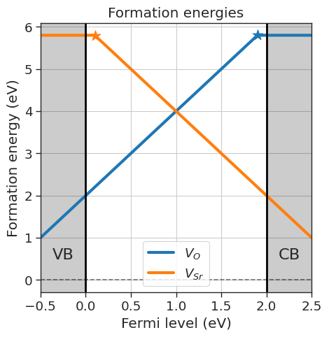
Let’s create an example DataFrame with made-up energies. We are studying $SrO$ and have energies for the neutral and charged $Sr$ and $O$ vacancies.

import pandas as pd
from defermi import DefectsAnalysis

bulk_volume = 800 # cubic Amstrong
data = [
{'name': 'Vac_O','charge': 2,'multiplicity': 1,'energy_diff': 7,'bulk_volume': bulk_volume},
{'name': 'Vac_O','charge':0,'multiplicity':1,'energy_diff': 10.8, 'bulk_volume': bulk_volume},
{'name': 'Vac_Sr','charge': -2,'multiplicity': 1,'energy_diff': 8,'bulk_volume': bulk_volume},
{'name': 'Vac_Sr','charge': 0,'multiplicity': 1,'energy_diff': 7.8,'bulk_volume': bulk_volume},
]
df = pd.DataFrame(data)
df

	name	charge	multiplicity	energy_diff	bulk_volume
0	Vac_O	2	1	7.0	800
1	Vac_O	0	1	10.8	800
2	Vac_Sr	-2	1	8.0	800
3	Vac_Sr	0	1	7.8	800

# Initialize DefectsAnalysis object
da = DefectsAnalysis.from_dataframe(df,band_gap=2,vbm=0) # band gap and valence band maximum in eV

import matplotlib.pyplot as plt

chempots = {'O':-5,'Sr':-2} # Define chemical potentials for each element in a dictionary

# Plot formation energies
da.plot_formation_energies(chemical_potentials=chempots,title='Formation energies',figsize=(5,5)).show()

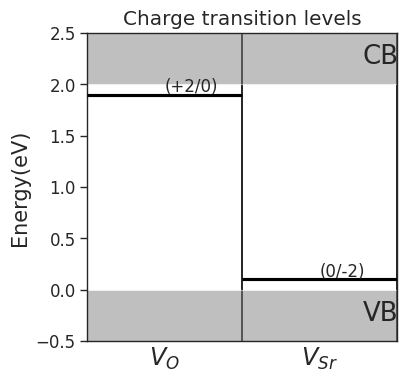
# Plot charge transition levels
da.plot_ctl(figsize=(4,4),fontsize=12)
plt.title('Charge transition levels');

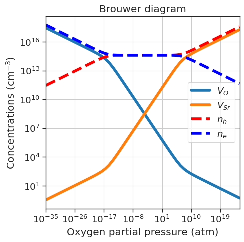
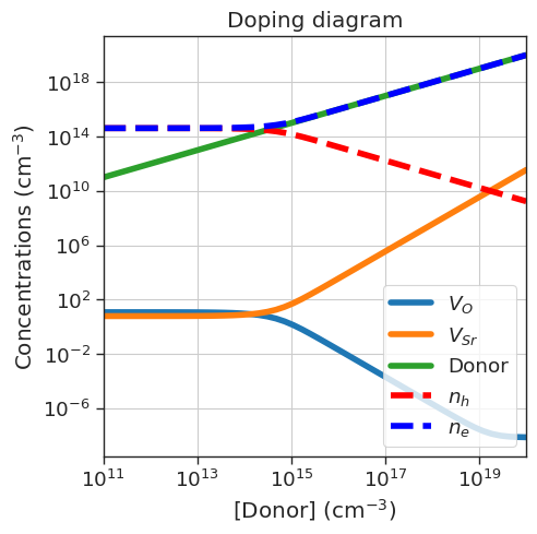
Fermi level dictated by charge neutrality

defermi also offers an easy way to study the defect equilibrium dictated by charge neutrality in different conditions. Defect concentrations can be plotted as a function of the oxygen partial pressure (Brouwer diagram) and dopant concentration (doping diagram) with one line of code.

# Brouwer diagram

precursors = {'SrO':-10} # Reservoir and energy p.f.u for the chemical potentials definition
oxygen_ref = -4.95  # chemical potential of oxygen at 0 K and standard pressure
bulk_dos = {'m_eff_e':0.5, 'm_eff_h':0.4}  # effective masses for the charge carriers calculation

da.plot_brouwer_diagram(
                    bulk_dos=bulk_dos,
                    temperature=1000, # Kelvin
                    precursors=precursors,
                    oxygen_ref=oxygen_ref,
                    pressure_range=(1e-35,1e25), # atm
                    figsize=(5,5))
plt.title('Brouwer diagram')
plt.show()

# Doping diagram

da.plot_doping_diagram(
                variable_defect_specie={'name':'Donor','charge':1},
                concentration_range=(1e11,1e20),  # cm^-3
                chemical_potentials=chempots,
                bulk_dos=bulk_dos,
                temperature=1000,  # Kelvin
                figsize=(5,5))
plt.title('Doping diagram');

This site is open source. Improve this page.